Создание функций распределения вероятностей (PDFs) из гистограмм
скажем, у меня есть несколько гистограмм, каждая с подсчетами на разные bin местоположения (на реальной оси). например,
def generate_random_histogram():

    # Random bin locations between 0 and 100
    bin_locations = np.random.rand(10,) * 100
    bin_locations.sort()

    # Random counts between 0 and 50 on those locations
    bin_counts = np.random.randint(50, size=len(bin_locations))
    return {'loc': bin_locations, 'count':bin_counts}

# We can assume that the bin size is either pre-defined or that
# the bin edges are on the middle-point between consecutive counts.
hists = [generate_random_histogram() for x in xrange(3)]
как я могу нормализовать эти гистограммы, чтобы получить PDF-файлы где Интеграл каждого PDF добавляет до одного в заданном диапазоне (например, 0 и 100)?
можно предположить, что гистограмма рассчитывает события на предопределенные ОГРН размере (например, 10)
большинство реализаций, которые я видел, основываясь, например, на Гауссова Ядра (см. scipy и scikit-learn), которые начинаются с данных. В моем случае мне нужно сделать это из гистограмм, так как у меня нет доступа к исходным данным.
обновление:
обратите внимание, что все текущие ответы предполагают, что мы смотрим на случайную величину, которая живет в (-Inf, +Inf). Это нормально, как грубое приближение, но это может быть не так в зависимости от приложения, где переменная может быть определена в некотором другом диапазоне [a,b] (например, 0 и 100 в данном случае)
3 ответов
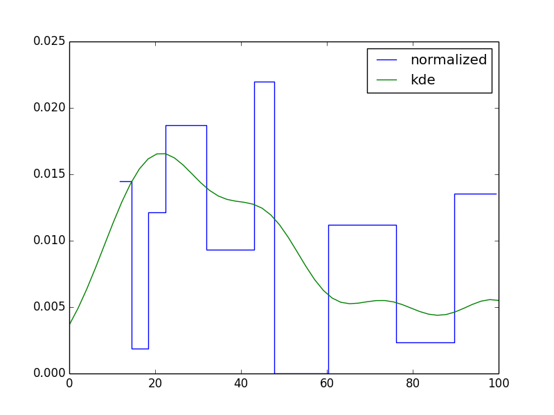
главный пункт деликатности определяет bin_edges поскольку технически они могут быть где угодно. Я выбрал среднюю точку между каждой парой мусорных центров. Вероятно, есть и другие способы сделать это, но вот один:
hists = [generate_random_histogram() for x in xrange(3)]
for h in hists:
    bin_locations = h['loc']
    bin_counts = h['count']
    bin_edges = np.concatenate([[0], (bin_locations[1:] + bin_locations[:-1])/2, [100]])
    bin_widths = np.diff(bin_edges)
    bin_density = bin_counts.astype(float) / np.dot(bin_widths, bin_counts)
    h['density'] = bin_density

    data = np.repeat(bin_locations, bin_counts)
    h['kde'] = gaussian_kde(data)

    plt.step(bin_locations, bin_density, where='mid', label='normalized')
    plt.plot(np.linspace(0,100), h['kde'](np.linspace(0,100)), label='kde')
что приведет к следующим графикам (по одному для каждой гистограммы):
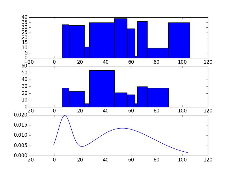
вот одна возможность. Я не в восторге от этого, но это вроде как работает. Обратите внимание, что гистограммы немного странные, так как ширина Бина довольно переменная.
import numpy as np
from matplotlib import pyplot
from sklearn.mixture.gmm import GMM
from sklearn.grid_search import GridSearchCV

def generate_random_histogram():
    # Random bin locations between 0 and 100
    bin_locations = np.random.rand(10,) * 100
    bin_locations.sort()

    # Random counts on those locations
    bin_counts = np.random.randint(50, size=len(bin_locations))
    return {'loc': bin_locations, 'count':bin_counts}

def bin_widths(loc):
    widths = []
    for i in range(len(loc)-1):
        widths.append(loc[i+1] - loc[i])
    widths.append(widths[-1])
    widths = np.array(widths)
    return widths

def sample_from_hist(loc, count, size):
    n = len(loc)
    tot = np.sum(count)
    widths = bin_widths(loc)
    lowers = loc - widths
    uppers = loc + widths
    probs = count / float(tot)
    bins = np.argmax(np.random.multinomial(n=1, pvals=probs, size=(size,)),1)
    return np.random.uniform(lowers[bins], uppers[bins])

# Generate the histogram
hist = generate_random_histogram()

# Sample from the histogram
sample = sample_from_hist(hist['loc'],hist['count'],np.sum(hist['count']))

# Fit a GMM
param_grid = [{'n_components':[1,2,3,4,5]}]
def scorer(est, X, y=None):
    return np.sum(est.score(X))
grid_search = GridSearchCV(GMM(), param_grid, scoring=scorer).fit(np.reshape(sample,(len(sample),1)))
gmm = grid_search.best_estimator_

# Sample from the GMM
gmm_sample = gmm.sample(np.sum(hist['count']))

# Plot the resulting histograms and mixture distribution
fig = pyplot.figure()
ax1 = fig.add_subplot(311)
widths = bin_widths(hist['loc'])
ax1.bar(hist['loc'], hist['count'], width=widths)
ax2 = fig.add_subplot(312, sharex=ax1)
ax2.hist(gmm_sample, bins=hist['loc'])
x = np.arange(min(sample), max(sample), .1)
y = np.exp(gmm.score(x))
ax3 = fig.add_subplot(313, sharex=ax1)
ax3.plot(x, y)
pyplot.show()
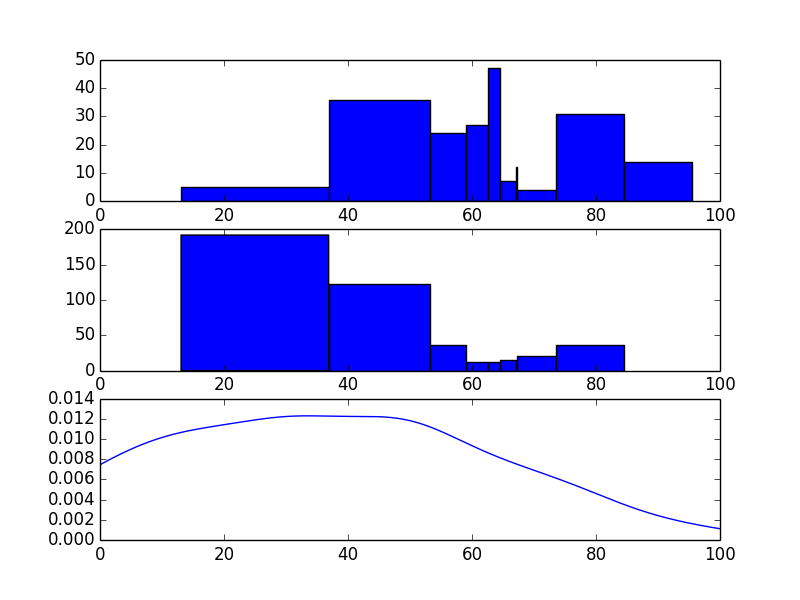
вот способ сделать это с pymc. Этот метод использует фиксированное количество компонентов (n_компонентов) в модели смеси. Вы можете попробовать прикрепить A до n_components и выборку над этим ранее. Кроме того, вы можете просто выбрать что-то разумное или использовать метод поиска сетки из моего другого ответа, чтобы оценить количество компонентов. В приведенном ниже коде я использовал 10000 итераций с записью 9000, но этого может быть недостаточно для получения хороших результатов. Я бы предложил использовать гораздо больший ожог. Я также выбрал priors несколько произвольно, так что это может быть что-то посмотреть. Вам придется поэкспериментировать с ним. Удачи вам. Вот код.
import numpy as np
import pymc as mc
import scipy.stats as stats
from matplotlib import pyplot

def generate_random_histogram():
    # Random bin locations between 0 and 100
    bin_locations = np.random.rand(10,) * 100
    bin_locations.sort()

    # Random counts on those locations
    bin_counts = np.random.randint(50, size=len(bin_locations))
    return {'loc': bin_locations, 'count':bin_counts}


def bin_widths(loc):
    widths = []
    for i in range(len(loc)-1):
        widths.append(loc[i+1] - loc[i])
    widths.append(widths[-1])
    widths = np.array(widths)
    return widths


def mixer(name, weights, value=None):
    n = value.shape[0]
    def logp(value, weights):
        vals = np.zeros(shape=(n, weights.shape[1]), dtype=int)
        vals[:, value.astype(int)] = 1
        return mc.multinomial_like(x = vals, n=1, p=weights)

    def random(weights):
        return np.argmax(np.random.multinomial(n=1, pvals=weights[0,:], size=n), 1)

    result = mc.Stochastic(logp = logp,
                             doc = 'A kernel smoothing density node.',
                             name = name,
                             parents = {'weights': weights},
                             random = random,
                             trace = True,
                             value = value,
                             dtype = int,
                             observed = False,
                             cache_depth = 2,
                             plot = False,
                             verbose = 0)
    return result

def create_model(lowers, uppers, count, n_components):
    n = np.sum(count)
    lower = min(lowers)
    upper = min(uppers)
    locations = mc.Uniform(name='locations', lower=lower, upper=upper, value=np.random.uniform(lower, upper, size=n_components), observed=False)
    precisions = mc.Gamma(name='precisions', alpha=1, beta=1, value=.001*np.ones(n_components), observed=False)
    weights = mc.CompletedDirichlet('weights', mc.Dirichlet(name='weights_ind', theta=np.ones(n_components)))

    choice = mixer('choice', weights, value=np.ones(n).astype(int))

    @mc.observed
    def histogram_data(value=count, locations=locations, precisions=precisions, weights=weights):
        if hasattr(weights, 'value'):
            weights = weights.value

        lower_cdfs = sum([weights[0,i]*stats.norm.cdf(lowers, loc=locations[i], scale=np.sqrt(1.0/precisions[i])) for i in range(len(weights))])
        upper_cdfs = sum([weights[0,i]*stats.norm.cdf(uppers, loc=locations[i], scale=np.sqrt(1.0/precisions[i])) for i in range(len(weights))])

        bin_probs = upper_cdfs - lower_cdfs
        bin_probs = np.array(list(upper_cdfs - lower_cdfs) + [1.0 - np.sum(bin_probs)])
        n = np.sum(count)
        return mc.multinomial_like(x=np.array(list(count) + [0]), n=n, p=bin_probs)

    @mc.deterministic
    def location(locations=locations, choice=choice):
        return locations[choice.astype(int)]

    @mc.deterministic
    def dispersion(precisions=precisions, choice=choice):
        return precisions[choice.astype(int)]

    data_generator = mc.Normal('data', mu=location, tau=dispersion)

    return locals()

# Generate the histogram
hist = generate_random_histogram()
loc = hist['loc']
count = hist['count']
widths = bin_widths(hist['loc'])
lowers = loc - widths
uppers = loc + widths

# Create the model
model = create_model(lowers, uppers, count, 5)

# Initialize to the MAP estimate
model = mc.MAP(model)
model.fit(method ='fmin')

# Now sample with MCMC
model = mc.MCMC(model)
model.sample(iter=10000, burn=9000, thin=300)

# Plot the mu and tau traces
mc.Matplot.plot(model.trace('locations'))
pyplot.show()

# Get the samples from the fitted pdf
sample = np.ravel(model.trace('data')[:])

# Plot the original histogram, sampled histogram, and pdf
lower = min(lowers)
upper = min(uppers)
kde = stats.gaussian_kde(sample)
x = np.arange(0,100,.1)
y = kde(x)
fig = pyplot.figure()
ax1 = fig.add_subplot(311)
pyplot.xlim(lower,upper)
ax1.bar(loc, count, width=widths)
ax2 = fig.add_subplot(312, sharex=ax1)
ax2.hist(sample, bins=loc)
ax3 = fig.add_subplot(313, sharex=ax1)
ax3.plot(x, y)
pyplot.show()
и, как вы можете видеть, эти два распределения не выглядят ужасно похожими. Однако гистограмма-это не так уж много. Я бы играл с разным количеством компонентов и большим количеством итераций / записи, но это проект. В зависимости от ваших приоритетов я подозреваю либо @askewchan, либо мой другой ответ мог бы послужить вам лучше.